Introduction to Using Microsoft Excel for Data Analysis - Sun and Planets Spirituality AYINRIN

From The Palace Of Kabiesi Ebo Afin!Ebo Afin Kabiesi! His Magnificence Oloja Elejio Oba Olofin Pele Joshua Obasa De Medici Osangangan broad-daylight natural blood line 100% Royalty The God, LLB Hons, BL, Warlord, Bonafide King of Ile Ife kingdom and Bonafide King of Ijero Kingdom, Number 1 Sun worshiper in the Whole World.I'm His Magnificence the Crown.
For Spiritual Consultations, Spiritual divination reading, Guidance and Counseling, spiritual products and spiritual Services, offering of Spiritual Declarations , call or text Palace and Temple Phone and Whatsapp contact: +2348166343145, Phone And WhatsApp Contact : +2347019686274 ,Mail: obanifa87@gmail.com, Facebook page: Sun Spirituality.Website:www.sunspirituality.com.
Our Sun spiritual Temple deliver Spiritual Services to Companies owners, CEOs, Business brands owners, Bankers, Technologists, Monarchs, Military officers, Entrepreneurs, Top Hierarchy State Politicians, and any Public figures across the planet.
Author:His Magnificence the Crown, Kabiesi Ebo Afin! Oloja Elejio Oba Olofin Pele Joshua Obasa De Medici Osangangan Broadaylight.
Excel is ubiquitous in the corporate world. A recent survey by Acuity Training revealed that office workers spend 38% of their time working in Excel.
This means that learning Excel is a very high ROI use of time – whether you read blog articles like this one, do an online course, or attend a structured Excel training course.
Primarily, Excel is a data aggregation and analysis tool. It transforms raw data into useful business insights. This post is a beginner’s post giving an introduction to using Microsoft Excel for data analysis.
1. Sorting Data
Sorting data is one of the basic processes in analyzing that data.
By sorting the data, you give your raw data a well-defined structure, and with structure, you can start to spot patterns in your data more easily.
Sorting data in Excel is simple. To show you how we’ll use an example data set below.
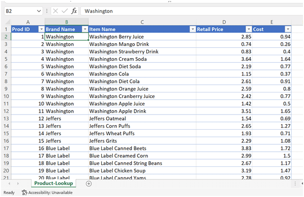
If your data is already formatted as an Excel table, as it is above, then you can quickly sort your data based on any column in the data.
But if the data is not formatted as a table, a couple of extra steps will be required.
See the below screenshot of our raw dataset below.
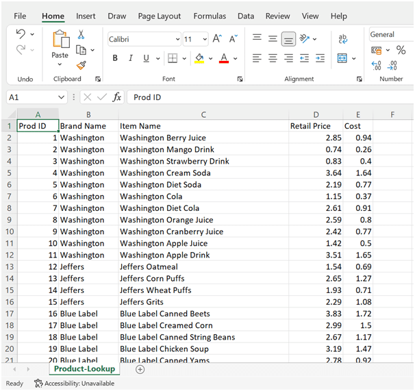
This will often be the case with datasets that you have imported into Excel whether it’s a .xlsx file or a CSV file.
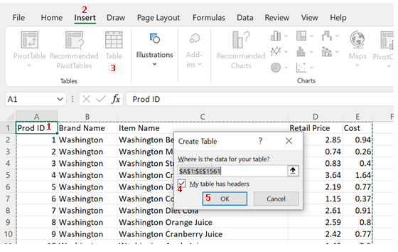
To convert this into a table:
- Select any cell in the data set. (1 in the screenshot below)
- Go to “Insert Tab” (2 below) and select Table. (3)
- By clicking on the table, Excel will automatically detect the range of the dataset and a new window will open showing the selected range.
- If your data already has column headers, then mark the option asking for data headers (marked as 4) and click OK.
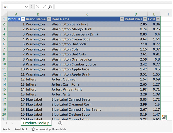
After clicking OK, your data will be converted into a table.
In the example below, we want to sort our data alphabetically using the second column “Brand Name” (marked as 1) and having a sorting order from A to Z (marked as 2).
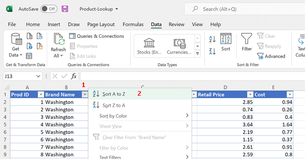
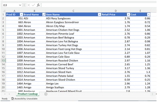
After clicking on “Sort A to Z”, the data will be arranged as shown below.
Besides the simple sorting option discussed above, Excel also offers more advanced features for re-arranging the data. You can sort the data based on multiple criteria and columns.
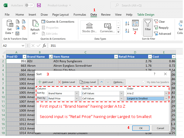
Let’s consider the above data again. Now we want to rearrange the data based on two columns, “Brand Name” and “Retail Price”.
To do this, select the Sort option (marked as 2) from the Data tab.
After clicking on Sort, a new window will pop up (marked as 3) where you can define the multiple levels for sorting the data. To do this you simply click ‘Add Level’ and define another filter.
If your data is properly formatted as a table, then Excel will automatically recognize the range for you while using this option.
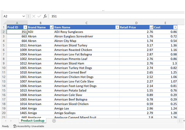
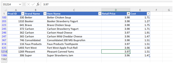
Now, the data will be arranged as shown below. As you can see, you aren’t limited to sorting on only two criteria. You can add further levels if you would like to carry out further analysis.
2. Filtering Data
Data filtering is a very useful process which helps to spot tends and outliers in datasets.
Filtering can also be used to derive quick insights from the data, like the top 10 products by price.
Excel offers a lot of options to filter data, including an extensive range of text and number filters. These filters can be used according to the type of data.
In the example below, we have used the number filter to filter out the top 10 products by the retail price.
If your data is formatted in a table, then you could find a small arrow for the drop-down menu on the right side of the top cell in each column (marked as “1” in the below picture).
But if your data is not formatted as a table and for some reason, you don’t want it to be a table, you can simply select all the headers of your data and apply filters by clicking on the “Filter” button under the “Data” tab.
A shortcut key to turn filters on is CTRL+Shift+L.
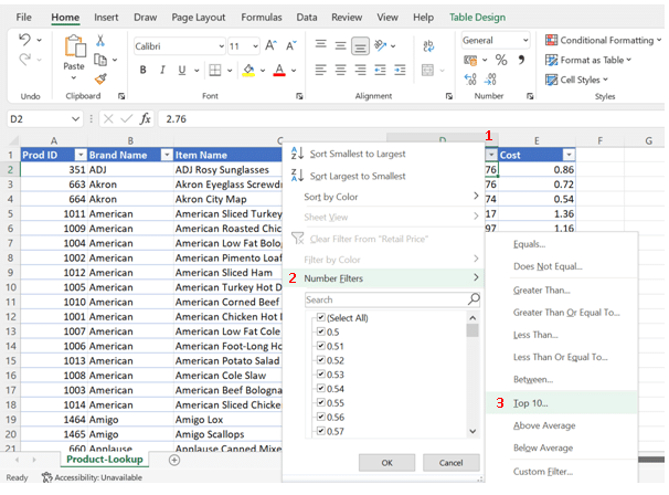
After clicking the “Top 10..” option (marked as 3), the data will be reduced to 10 products with the topmost retail prices.
In Excel, filters can also be used to process textual information. For example, if in the above data, we want to see all the yogurt-related items, then text filters can be used.
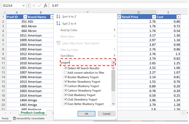
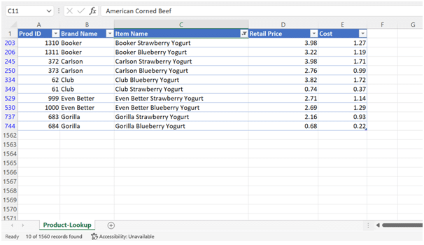
By typing “Yogurt” in the text field, all the products except yogurt will be filtered out from the list.
Other options in the Filter menu are quite helpful when you need to see the data set from different perspectives.
3. Conditional Formatting
Conditional formatting is used to highlight values based on certain criteria.
When you need to process multiple rows to search for specific values, conditional formatting can be a great help.
Conditional formatting can be used with numerical and text information.
Again, Excel offers multiple options.You can use the pre-built rules to highlight the cells, or you can define a custom rule that best fits your data.
In the below example, we want to highlight values where the margin value is between $1.5 to $2.
You can access the Conditional Formatting menu (marked as 2) under the Home tab (marked as 1).
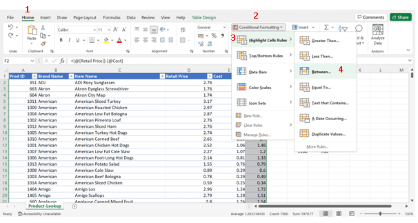
Next select ‘Highlight Cells Rules’ (marked as 3), and then click the “Between” option (marked as 4).
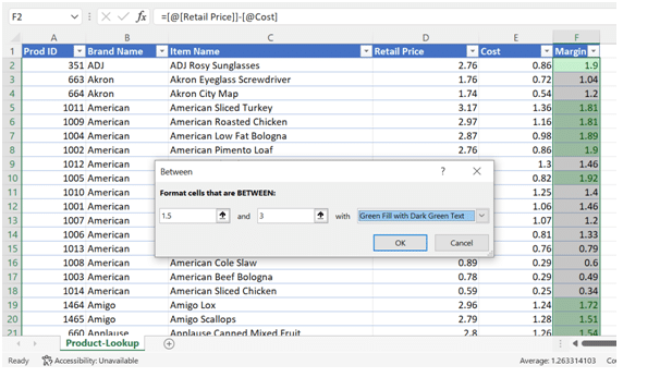
A new window will now appear (see screenshot below), which allows you to set the range of values that you want to highlight. In this case, values from $1.5 to $2 are highlighted.
While entering the value in the window, you can see the results being applied to your data providing a sort of preview.
Another example of using conditional formatting is to use the option of data bars to better visualize your data and give a more appealing look to your reports.
In our example, we might want to apply data bars to the margin column to visualize our results.
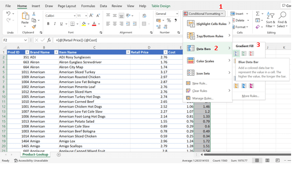
To apply data bars in the “Margin” column, first, select the entire column and then select “Data Bars” (marked as 2) from the conditional formatting menu (marked as 1).
In the “Data Bars” menu, you can select from different variations of solid fill and gradient fill (marked as 3).
After selecting your desired fill option (again Excel gives you a preview), data bars will be applied to the column.
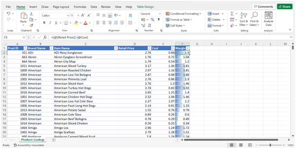
You can use the different options in conditional formatting to give your report a more appealing look or to increase the visibility of certain values in your data set.
Try and explore the remaining options to get a firm grip on using Conditional Formatting for different needs.
Final Thoughts
Microsoft Excel offers huge flexibility and freedom to carry out detailed data analysis. Learning the correct ways to do this will make these tasks quick and simple. Once you’ve mastered these basics, you can move on to more advanced data analysis like creating graphs.
Was this article helpful? Connect with me.


No comments:
Post a Comment
Note: Only a member of this blog may post a comment.